Configure the hysteretic core model of the LTspice simulator
| ©2004 Valentyn Volodin |
|
Unlike the Jiles–Atherton model, which is now used in most commercial SPICE simulators, the LTspice hysteretic core model uses the magnetic hysteresis loop parameters listed in Table 1 as settings.
| Parameter | Description | Units |
|---|---|---|
| Hc | Coercive force | A/m |
| Br | Remnant flux density | T |
| Bs | Saturation flux density | T |
 The model parameters enumerated in table 1 have a simple and understandable physical meaning. In addition, the hysteretic core model is distinguished by the fact that it quite adequately reproduces both limiting and partial magnetization reversal cycles of ferromagnetic materials.
However, in spite of a simple and small set of parameters, the hysteretic core model still requires a certain adjustment procedure. When modeling a ferromagnetic core operating in strong magnetic fields, it is important that the model adequately imitates core saturation as well as specific magnetic losses. Nevertheless, there are difficulties with the choice of parameters. The fact is that the saturation level of the hysteretic core model is set by the parameter Bs. It determines the limiting value to which the induction tends, if the magnetic field tends to infinity (without taking into account the component μ0H). In its reference data, the manufacturer also indicates the saturation induction Bs, which, however, is not a limiting value of induction. Usually, the induction corresponding to a large (for example, 1200 A/m), but not infinitely large, magnetic field strength is indicated as Bs. Using this parameter to configure the model will cause the model to saturate earlier than the actual ferromagnetic material.
The parameters Hc and Br are simultaneously used in the model to set the hysteresis and approximate the magnetization curve in the section with induction B ≤ Br. Despite that, in reality the properties of the ferromagnetic material are more important working in strong fields (the part of the magnetization reversal curve in the bend region) rather than in the field with induction B ≤ Br. Besides, the manufacturer indicates the values of Hc and Br for a specific case in his reference data (for example, for a magnetization reversal frequency of 10 kHz). Using these parameters to adjust the model, at least, will result in the model not correctly simulating the magnetization reversal losses if the ferromagnetic material is used at a different frequency.
Earlier, I gave a methodology for manually selecting the settings for the hysteretic core model. However, the use of this technique leads to a waste of time. The proposed calculator allows you to avoid time-consuming actions, as well as improve the accuracy of the model settings. The source data for this calculator are reference data, which are usually provided by manufacturers.
For example, let us have a look at N87 Epcos ferrite. Let us suppose that we are going to use this ferrite in the core of the transformer resonant LLC converter, where it will be magnetically reversed from -0.2 T to 0.2 T with a frequency of 100 kHz. It is assumed that the temperature of the ferrite core will reach 100° C.
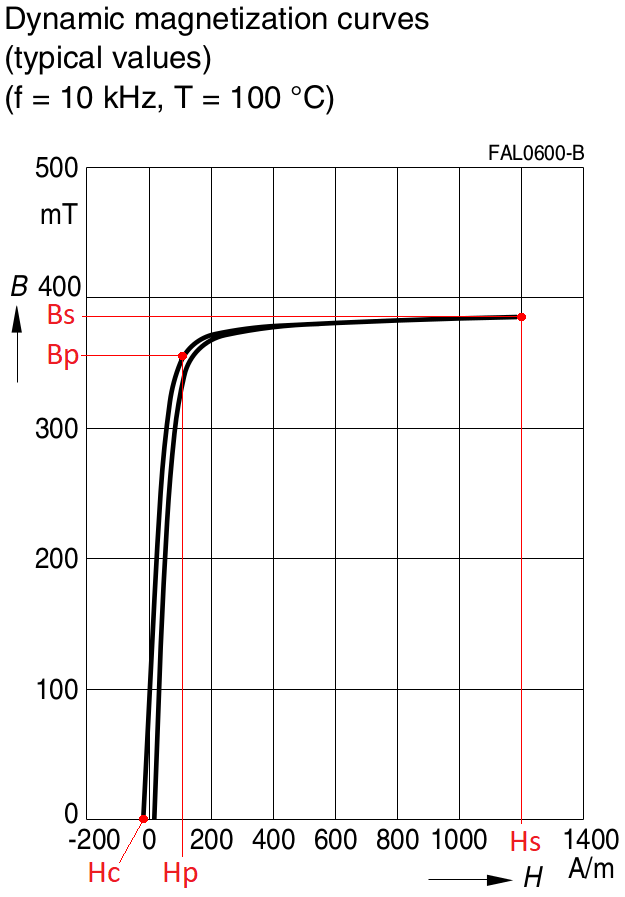
In the reference data, the manufacturer gives the form of dynamic hysteresis loops for temperatures of 25° C and 100° C obtained at a magnetization reversal frequency of 10 kHz. We select a graph for a temperature of 100° C. As initial data for the calculator, we can use both the upper and lower sections of the hysteresis loop. Let us use the top section. In this section, we need to select three points and determine their coordinates. The first point is located at the point where the curve intersects the abscissa axis (B = 0) and, accordingly, has the coordinates Hc : B = 0. The second point is located in the bend region of the upper section and has the coordinates Hp : Bp. The third point is located in the region of maximum induction and has the coordinates Hs : Bs. We define the coordinates of these points from the graph:
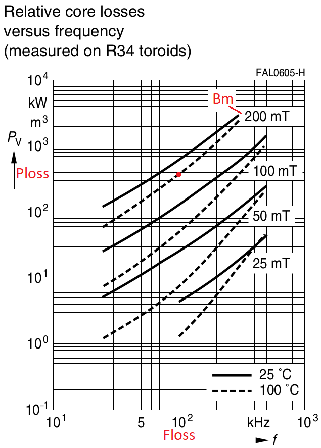
Hc = -16.5 A / m; Hp = 109 A / m: Bp = 0.356 T; Hs = 1200 A / m: Bs = 0.39 T. Next, we determine the losses for the case of core magnetization reversal with a frequency of Floss = 100 kHz, maximum induction Bm = 0.2 T, and a temperature of 100° C. Using the manufacturer's graphical data, we estimate the losses for these conditions Ploss = 376 kW / m3.
We enter the source data in the appropriate cells of the calculator and click on the button "Count". The calculator gives a line of model parameters:
Hc = 8.9816 Br = 0.15745 Bs = 0.39433